
Principle of magnetotelluric method
Preface
In this page, the principle to obtain conductivity structure in the Earth's interior, so called magnetotelluric (MT) method, is introduced. Note that this page is written by a non-specialist of MT survey for non-specialists people. If you find any problem, please let me know it.
Principle
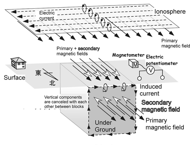
Electric current in ionosphere -> primary magnetic field
Primary magnetic field -> induced current under ground
Current under ground -> secondary magnetic field
Observation of primary + secondary magnetic fields and of electric potential
Magnitude of electric current induced by primary magnetic field: a function of conductivity under ground.
Observation system
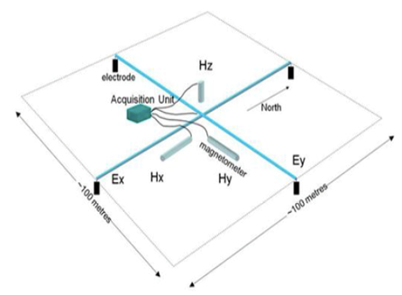
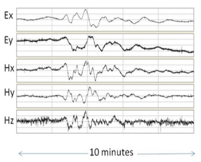
Measuring field components:
Magnetic field: x, y z components (Hx, Hy, Hz)
Electric field: x, y components (Ex, Ey)
Physical Basis of MT survey
Basic equations
Faraday's law: electric field is generated by time variation of magnetic field
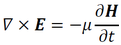
(1)
E: electric field
H: magnetic field
𝜇: magnetic permeability
Ampere's law: a magnetic field is generated by electric current and time variation of magnetic field.
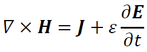
(2)
J: electric current density
𝜀: magnetic permeability
Electric current. The current density is proportional to the electrical conductivity and the electric field.

(3)
𝜎: electric conductivity
Time variation of electromagnetic field is considered a series of harmonic oscillations. As is usual, each harmonic oscillation is expressed by a complex function exp(iωt).
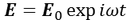
(4)
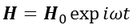
(5)
𝜔: angular frequency
𝑖: imaginary unit
Time derivatives of these function (Eq. 4 and 5) are given by multiplying them by iω.
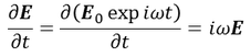
(6)
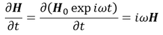
(7)
The time derivatives of oscillating electric and magnetic fields are proportional to the magnitude of the oscillating fields and their frequencies.
The multiplication by the imaginary unit means that the phases of the time derivatives are by 1/4 cycle advanced to the oscillation of the fields.
One-dimensional structure
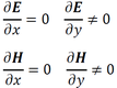
Here, we argue one-dimensional conductivity structures, which is homogeneous in horizontal directions.
These conditions are expressed by the following equations.
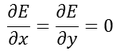
(8)
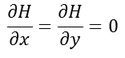
(9)
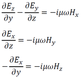
Three components of Fraday's law (Eq. 1)
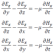
(10)
By substituting Eqs. (6) and (8) into Eq. (10)
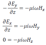
(11)
The vertical component of magnetic field is zero.
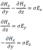
Three components of Ampere's law (Eq. 2) with the equation of electric current (Eq. 3)
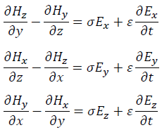
(12)
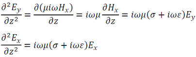
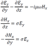
By substituting Eqs. (7) and (9) into Eq. (12), we have.
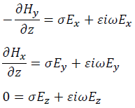
(13)
Eq. (13) is simplified as
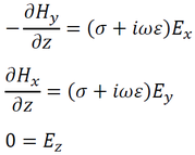
(14)
The vertical component of the electric field is zero.
By combining Eqs. (12) and (14), we have
(15)
By substituting k2 = iωμ(σ + iωε) into Eq. (15), we have
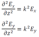
(16)
Here, we have
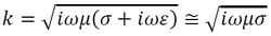
(17)
because
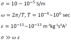
(18)
The inequality σ ≫ ωε means the secondary magnetic field is generated by electric current under ground but not by oscillation of the electric field.
The differential equations Eqs. (16) and the compolex number of k given by (17) indicate that both x and y components of the electric field oscillate and exponentially attenuate with depth (z). Together with Eq. (6), we have
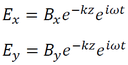
(19)
Similarly, we have the following equation for the magnetic field:
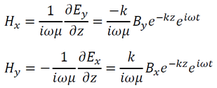
(20)
Here the impedance tensor Zij is defined by Zij = Ei/Hj.
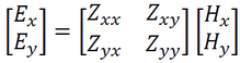
(21)
From the definition, the components Zxy and Zyx are:
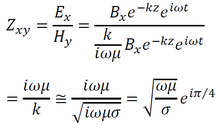
(22)
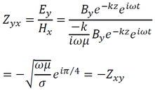
(23)
The factor eiπ/4 means that the phase of the electric field is by 1/8 cycles advanced.
We can obtain "apparent" conductivity from Eqs. (19) and (20) as
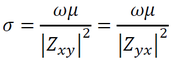
(24)
Thus, we can obtain conductivity under ground by comparing the magnitude of electric field to magnetic field.
Finally, the diagonal component of the impedance matrix should be zero,
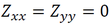
(25)
because the x components of the electric and magnetic fields do not induce the other one, and this is also the case for the y components.
Skin depth
Electromagnetic waves attenuate according to Eqs. (18) and (19). This attenuation is caused by electric flow by induction under ground. Therefore, MT survey provides conductivity values to limited depths. The depth where amplitude of electromagnetic wave becomes 1/e ≈ 0.37 to that at the surface is called "skin depth", δskin. The real part of the exponent e-kz in Eqs. (18) and (19) must be -1 at this depth. Namely, the skin depth is reciprocal Re(k). From Eq. (17), we therefore have:
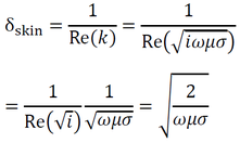
(26)
The skin depth decreases with increasing frequency. By obtaining apparent conductivity at different frequencies, we can obtain a conductivity profile with depth.
It is also noted that it decreases with increasing conductivity. This means that the surveyed region is shallower if conductivity is high.
Two-dimensional structure
Let us consider a structure that is uniform in x-direction but not in y-direction. In this case, conditions of Eqs. (8) and (9) are not held. Instead,
(27)
Under these conditions, Eq. (1) with Eq. (7) becomes
(28)
Similarly, Eq. (2) with Eq. (6) becomes
(29)
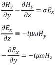
The 1st equation in Eqs (28) and the 2nd and 3rd equations in Eqs (29) contains Hx, Ey and Ez but not others. Therefore we make a set of these three equations, which is called TM mode.
(30)
From Eqs. (30), we have a Helmholtz equation of Hx only.
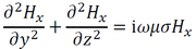
(31)
The other equations in Eqs (28) and (29) contain Ex, Zy and Zz, but not others. Therefore, we make a set of these three equations, which is called TE mode.
(32)
From Eqs. (32), we have a Helmholtz equation of Ex only.
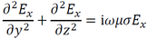
(33)
We can obtain two-dimensional conductivity profiles by inverting Eq. (31) (TM mode) and Eq. (33) (TE mode) independently.